感知机
感知机是一种监督学习算法 ,用于解决线性可分(Linearly Separable)的二分类问题,具体内容如下:
计算预测值:$z=w_1x_1 + w_2x_2 + b$
激活函数为阶跃函数:
$$
y_{pred}=
\begin{cases}
1 & z \ge 0\\
0 & z \lt 0
\end{cases}
$$
参数更新函数:
$$
w_i = w_i + \eta \cdot (y_{true} - y_{pred}) \cdot x_i$$
$$b = b + \eta \cdot (y_{true} - y_{pred})$$
下面我们通过具体的例子,应用一下上面的公式来使用感受一下:
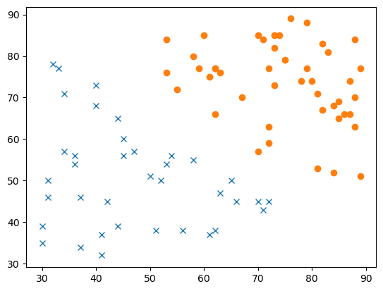
学生有两门课程的成绩,语文和数学,预测是否通过考试
假设每科分数均为 0-100,同时总分超过 120 分为通过考试
构造测试数据
1
2
3
4
5
6
7
8
9
10
11
12
13
14
15
16
17
18
19
20
21
22
23
24
25
import numpy as npimport matplotlib.pyplot as pltnum_samples = 50 X_1 = np.random.randint(30 , 80 , size=(num_samples, 2 )) X_fail = X_1[(X_1[:, 0 ] + X_1[:, 1 ] < 120 )] X_2 = np.random.randint(50 , 90 , size=(num_samples, 2 )) X_pass = X_2[(X_2[:, 0 ] + X_2[:, 1 ] >= 120 )] train_x = np.vstack([X_fail, X_pass]) train_y = np.array([0 ] * len (X_fail) + [1 ] * len (X_pass)) plt.plot(train_x[train_y == 0 ][:, 0 ], train_x[train_y == 0 ][:, 1 ], 'x' ) plt.plot(train_x[train_y == 1 ][:, 0 ], train_x[train_y == 1 ][:, 1 ], 'o' ) plt.show()
对应图如下:
数据预处理
主要对数据进行一下标准化
1 2 3 4 5 6 7 8 9 10 11 mu = train_x.mean(axis=0 ) sigma = train_x.std(axis=0 ) def standardize (x ): return (x - mu) / sigma X = standardize(train_x) y = train_y
开始训练
1 2 3 4 5 6 7 8 9 10 11 12 13 14 15 16 17 18 19 20 21 22 23 24 25 26 27 28 29 30 leaning_rate = 0.1 max_epochs = 200 weights = np.random.randn(2 ) * 0.01 bias = 0 for epoch in range (max_epochs): has_error = False for i in range (len (X)): z = np.dot(X[i], weights) + bias y_pred = 1 if z >= 0 else 0 if y_pred != y[i]: weights += leaning_rate * (y[i] - y_pred) * X[i] bias += leaning_rate * (y[i] - y_pred) has_error = True if not has_error: break print (f"weights={weights} , bias={bias} " ) accuracy = np.mean([1 if np.dot(X[i], weights) + bias >= 0 else 0 for i in range (len (X))] == y) print (f"Epoch {epoch} , Accuracy: {accuracy} " )
输出结果如下
1
2
3
4
5
6
weights=[0.16655886 0.06095784], bias=0.1 Epoch 0, Accuracy: 0.9024390243902439 weights=[0.16064312 0.14377813], bias=0.1 Epoch 1, Accuracy: 0.9512195121951219 weights=[0.26445705 0.25942353], bias=0.0 Epoch 2, Accuracy: 1.0
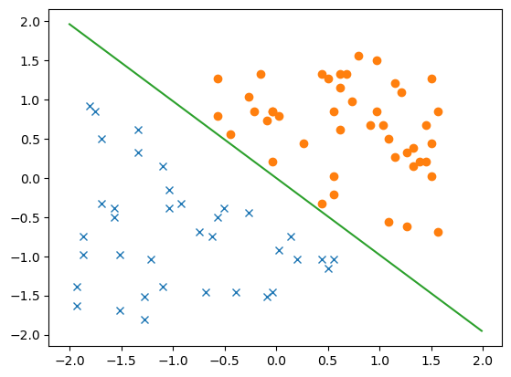
可以得到$0.26445705 x_1+0.25942353 x_2=0$,下面将这条分界线画出来
1 2 3 4 5 6 7 plt.plot(X[y == 0 ][:, 0 ], X[y == 0 ][:, 1 ], 'x' ) plt.plot(X[y == 1 ][:, 0 ], X[y == 1 ][:, 1 ], 'o' ) xx = np.arange(-2 , 2 , 0.01 ) plt.plot(xx, -weights[1 ] / weights[0 ] * xx) plt.show()
对应结果
此时预测函数可以如下定义
1
2
def predict (X ): return np.dot(X, weights) + bias >= 0
最后我们再自己构造数据进行验证也查下
1 2 3 4 5 6 data = [[60 , 70 ], [80 , 90 ], [50 , 50 ], [70 , 80 ]] stand_data = standardize(data) predict(stand_data)
输出结果如下,符合预期
1 > array([ True, True, False, True])